getting text that appears after a specific character
There are TextBefore & TextSplit formulas too!
When to Use the TEXTAFTER Formula
When you need to get data that appears after a specific character in a cell
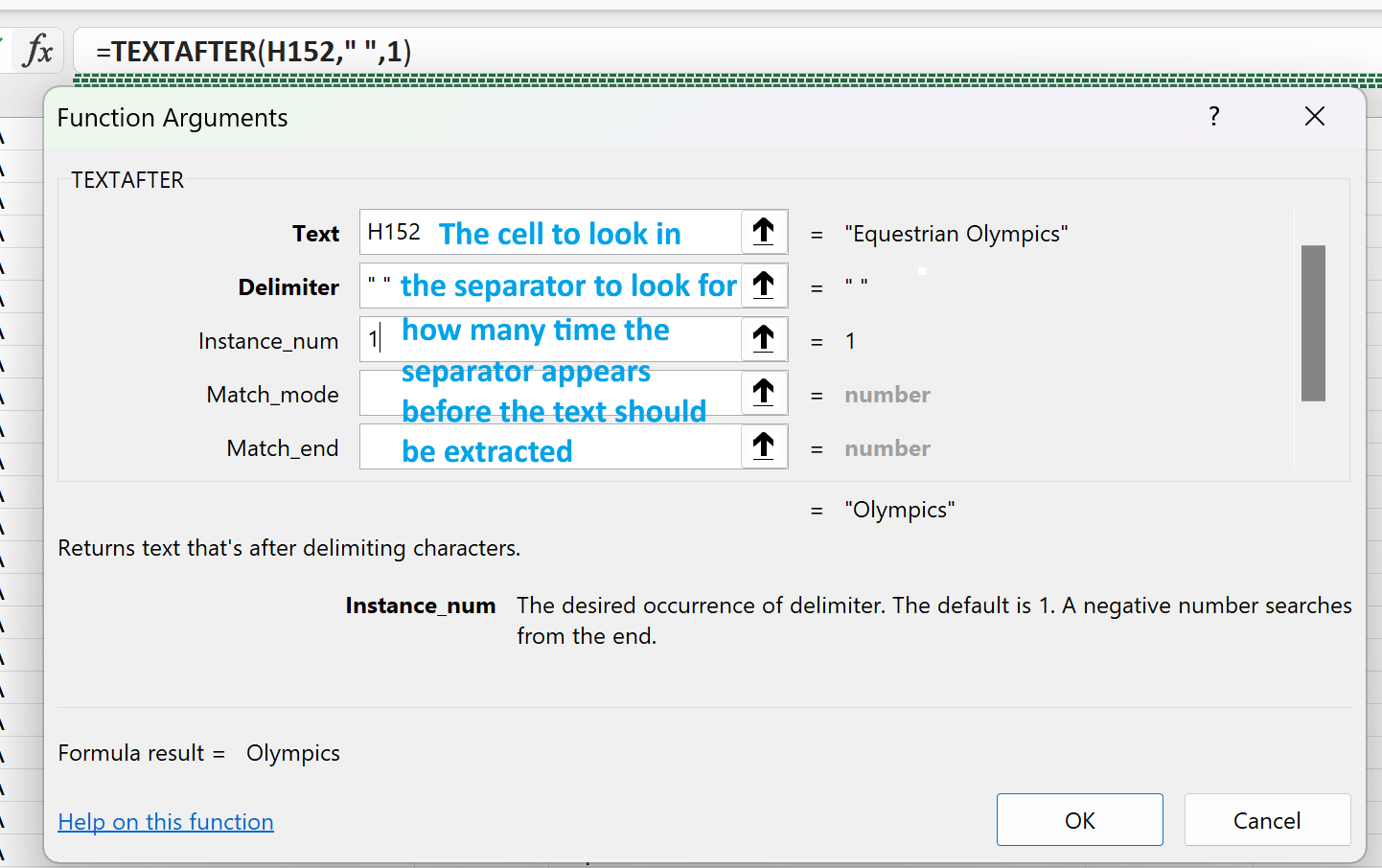
Mandatory Components of the TEXTAFTER Formula
Text: Which cell or range the formula should look in for the initial data (H152)
Delimiter: What character the formula should look for (a space)
Instance Number: How many times does the delimiter appear before the text should be extracted? (1)
- If there were 2 spaces in the cell before the text we wanted to extract the number would be 2
Excel formula: extract text after character
To extract the text that appears after a specific character, you supply the reference to the cell containing the source text for the first (text) argument and the character in double quotes for the second (delimiter) argument.
For example, to extract text after space the formula is:
=TEXTAFTER(A2, " ")
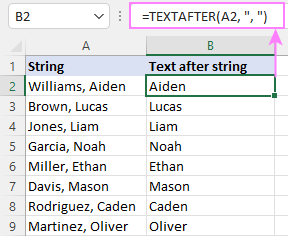
Excel formula: get text after string
To return the text that occurs after a certain substring, use that substring for the delimiter.
For example, if the last and first names are separated by a comma and a space, use the string ", " for delimiter:
=TEXTAFTER(A2, ", ")
Excel formula: extract text after word
In Excel terms, a "word" is nothing else but a "substring". So, to copy text after a specific word into another cell, specify the word as the delimiter.
For instance, to get the text after the word "color", use this formula:
=TEXTAFTER(A2, "color ")
Please note that the delimiter includes a space after the word "color " to avoid leading spaces in the results.
Now that you've got a grasp of the basics, let's investigate a few more complex scenarios.
Return text after Nth occurrence of delimiter
To get text that appears after the nth instance of the delimiter, make use of the instance_num parameter.
For example, to extract the text after the second comma, you use the string ", " for delimiter and the number 2 for instance_num:
=TEXTAFTER(A2, ", ", 2)
Again, the delimiter includes a space because, in the original text, the values are separated by a comma and a space.
Get text after last occurrence of delimiter
To extract the text after the last occurrence of the delimiter, use a negative value for the instance_num argument.
For example, to return the text after the last comma in A2, set instance_num to -1:
=TEXTAFTER(A2, ", ", -1)
To extract the text after the last but one comma, set instance_num to -2:
=TEXTAFTER(A2, ", ", -2)
Get text after multiple delimiters
To handle multiple delimiters at a time, you can use an array constant like {"x","y","z"} in your TEXTAFTER formula, where x, y, and z are different characters or substrings.
For instance, in the dataset below, the delimiter is either a comma or semicolon, with or without a space. To handle all four variations of the delimiter correctly, we use the array constant {",",", ",";","; "}:
=TEXTAFTER(A2, {",",", ",";","; "})
If delimiter not found, return your own text
If the TEXTAFTER function cannot match delimiter in the original text string, it returns a #N/A error by default. In many situations it makes more sense to output a custom value instead. For this, you need to define the if_not_found argument (the last one).
For example, if the word "color " does not exist in cell A2, this formula would throw a #N/A error:
=TEXTAFTER(A2, "color ")
To return a blank cell instead, we supply an empty string ("") for if_not_found:
=TEXTAFTER(A2, "color ", , , , "")
Alternatively, you can type any text or character you want, say a hyphen "-":
=TEXTAFTER(A2, "color ", , , , "-")
If delimiter is not found, return original text
To return the original text every time the TEXTAFTER function cannot match the delimiter, this is what you need to do:
- Set instance_num to -1 to search the source string from right to left.
- Set match_end to 1 to treat the end of the string as the delimiter.
When searching backwards, the beginning of the string becomes the "end", so the formula returns the entire text when the delimiter is not found.
In our case, the delimiter is a substring consisting of a colon and a space:
=TEXTAFTER(A2, ": ", -1, ,1)
If the delimiter is not present in a given cell, the entire cell contents are returned.
TEXTAFTER formula case-sensitive and case-insensitive
By default, the Excel TEXTAFTER function is case-sensitive, treating lowercase and uppercase delimiters as different ones. To make the formula case-insensitive, set the match_mode argument to 1 or TRUE.
For example, the below formula only accepts the lowercase "color " as the delimiter:
=TEXTAFTER(A2, "color ")
To make the formula case-insensitive, so it accepts the word-delimiter regardless of the letter case, we set the match_mode argument to 1:
=TEXTAFTER(A2, "color ", ,1)
Excel TEXTAFTER function not working
If the function does not exist in your Excel, please check out TEXTAFTER availability.
If the function results in an error, it's most likely to be one of these reasons:
A #N/A error occurs when:
- The delimiter is not found the source string. To fix the error, configure the if_not_found argument as explained in this example.
- The instance_num value is higher than the total number of the delimiters in text.
A #VALUE! error occurs when:
- The instance_num argument is set to 0.
- The instance_num value is higher than the total length of text.

